In inferential analysis you are answerable about the likelihood of happening certain event with respect to certain time e.g. Predicting what types of people will eat a diet in good quality during the next year. After answering this question using your model, you communicate your findings to your stake holders i.e. what factors make these people will eat high fresh diet, these factors help in your stake holders taking some measurable decision. If you can’t tell factors precisely using your model then there will be no action in the business and a question may be asked ”SO WHAT?” What business problem it is going to solve?
Regression models fails to deliver good intuition with the data sets if there is high correlation between independent variables, high correlation is good between dependent and independent variables but not between independent variables, if they are moderate (not high between independent variables) then its fine.
One of the regression model assumption is none of the independent variables should be constant, and there should not be an exact linear relationships among the independent variables, Highly Correlated independent variable are exact linear in relation with each other and these Highly Correlated independent variables in a model is called Multicollinearity, this is one of the problem in regression model which can make your model less interpret able and can increase standard error of your predictor variable’s coefficient estimate. There are always some Correlation between independent variables because this is the reason multiple regression came into existence, this correlation help to infer causality in cases where simple regression analysis (with one independent variable) can’t, but the same is bad if there is high correlation exist between independent variable
Here I am aiming only to describe how miss interpretation and increasing standard error in the model coefficient estimate occurs due to multicollinearity. We all now aware multicollinearity arises when two predictor variables are highly correlated in a model, such as high income in certain people influence to take high fresh diet or probably the more aged people influence them to take high fresh diet. If your model can’t detect which is exactly influencing people to take high fresh diet then your business stake holders cannot manifest the spot to increase the sale.In short with high multicollinearity it is very difficult to draw ceteris paribus conclusion about income or people age affects on high fresh diet
Standard error of a coefficient tell us how much sampling variation there is if we were to re-sample and re-estimate the coefficients of a model. So question comes here why highly correlated variable (multicollinearity) increase Standard error of their coefficient estimate? The more highly correlated independent variables are, the more difficult it is to determine how much variation in outcome variable is due to each these correlated independent variables. For example, in our example set if high income and age are highly correlated (which means they are very similar to each other) it is difficult to determine whether high income is responsible for variation in buying good quality food or ages of aged people, as a result , the standard errors for both variables become very large
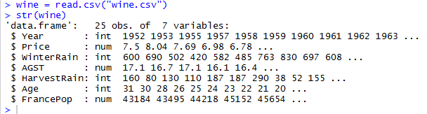
I will take an example data set from wine industry where many different variables that
could be used to predict wine price e.g. average growing season temperature (AGST), harvest rain, winter rain ,age of wine, population of France where this wine is producing etc.
I will use R here to depict multicollinearity and its effect on estimated coefficient standard error
Here i am going to check which predictor variables are highly correlated (remember correlated predictor variables are the fancy name of multicollinearity) using data visualization – A part of an Exploratory data analysis tool , visualizing is the most important tool for exploratory data analysis because the information conveyed using graphs can be very intuitive to recognize pattern. Highly correlated variables are those whose absolute value of correlation is close to 1.
I am here just randomly checking the correlation between AGST and HarvestRain

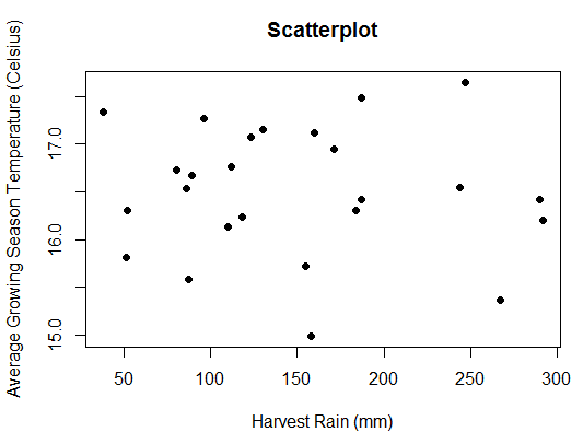
Hard to visually see a linear relationship between AGST and HarvestRain, and it turns out that the correlation between these two variables are close to 0 hence no correlation

Rather finding correlation between predictor variables one by one we can find the same between all variables within any data set in one go

Here you can see using above data matrix that Age and FrancePop are highly negative correlated as it is very close to 1, we can validate it by plotting graph


Hence it is proved that variable FrancePop and Age has strong correlation and will have multicollinearity problem, if these two variables will be the part of model then these will mislead to interpret the model to find which one actually predicting wine price
In this situation we need to get rid of one insignificant variable in order to make our model precise interpret-able. Before going to remove one insignificant variable we need to understand increasing the standard error of coefficient estimate of these two variables coefficient estimate due to multicollinearity
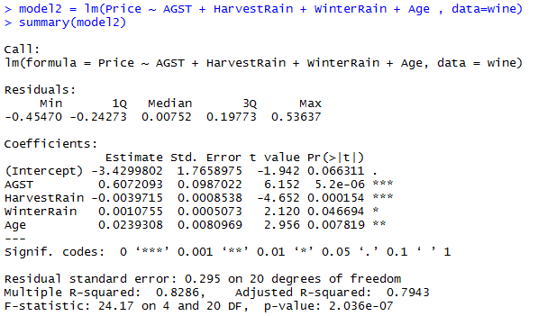
Lets create a model which include all the independent variables

As you can see highlighted standard error of Age and FrancePop variable in model has more noise with two standard error Age 0.07900 and FrancePop 0.0001667. These two variables doing the same task predicting wine price which is redundant and an extra noise, this extra noise make the estimates very sensitive to minor changes in the model. The result is that the coefficient estimates are unstable and difficult to interpret. Coefficients may have the “wrong” sign or implausible magnitudes e.g. -4.953-05
Above standard error magnitude can easily trick you as FrancePop magnitude is less than Age magnitude so FrancePop is more significant, but this is not the way to find which one is less unstable. There is a way to find more significant or less unstable variable between these two correlated variable and this is called VIF (Variable Inflation factor)
Highest VIF variable is a sign of best candidate to be removed from the model, threshold value for the VIF is greater than 5 and it depends on your model usage and its application see detail for VIF threshold VIF Threshold common practice if any correlated variable has greater than 5 VIF or whichever is bigger are deemed to be removed from the model

As you can see the Age and FrancePop both has VIF greater than 5 but Age VIF is less than FrancePop. We expect Age to be significant as older wines are typically more expensive,so Age makes more intuitive sense in our model
Now see the standard error of Age when FrancPop was with it in previous model
0.07900>0.00809
standard error rate of Age has been decreased, not only Age standard error decreased the other independent variable’s standard error decreased as well e.g. AGST standard error is now 0.0987011 while with these two correlated variable (Age+FrancePop) in model1 was 1.030e-01 = 0.1030 , same as with HarvestRain decreased from 8.751e-04 = 0.0008751 to 0.0008538 ,would you mind notice other factors as well Age has been more significant in model2 as compare to model1 (with FrancPop) and over all p-value of model is now 0.0000002036 which was 0.000001044 in model1
Lets see what happens if we drop Age variable and keep FrancePop

As you can see by dropping Age variable and including only FrancePop cause WinterRain variable less significant
In all above workaround , notice the R-squared value almost 82% in all cases with Age and FrancePop or with only Age or with only FrancePop R-squared value remains 82%, this R-squared is telling us how well our model is fitting the data , but we can’t say each of them is giving us accurate predictions , to find the accuracy of each model we need to run a cross validation to measure the accuracy of above each workaround
Caveats
- Dropping any important variable can lead your regression model to bias i.e. jumping your model from multicollinearity to heteroscedasticity problem (dependent variable became correlated with the error term), see below figure where bias is estimated parameter E(B^) to population parameter (true B), an unbiased estimator will come into your model
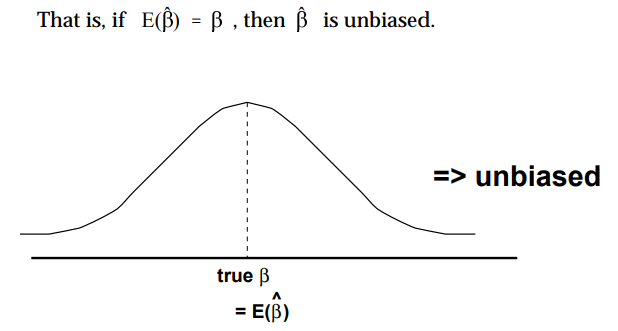
If E(B^) is not equal to (true B) then biased
- Increasing standard error for the estimated coefficient cause increasing confidence interval not making an estimated variable coefficient biased
- Do not put in too many variables in your model blindly put in place EDA to check variables that measure the same thing
Conclusion
In short Multicollinearity effect intuition of overall model by increasing standard error of each independent variable coefficient estimate which often result in non significant result (P-Value) and one of correlated coefficients may have the non sensual direction
Multicollinearity can occur if you accidentally include the same variable twice, e.g. height in inches and height in feet. Another common error occurs when one of the variable is computed from the other variable (e.g. Family income = Wife’s income + Husband’s income). EDA is very crucial step before creating any model,it can determine if there are any problems with your dataset and is the business question you are trying to solve can be answerable by the data you have in place
